Table of Contents
Lab 10 - Simulating Robot Localization
Now that the robot is capable of mapping its global environment, as demonstrated in Lab 9, it is time to implement localization. For this lab, the localization will take place in a simulated virtual environment. Robot localization allows a robot to map its immediate surroundings to determine its position within a global map.
To execute localization, we use the Bayes Filter. This filter incorporates sensor data, control inputs, and the robot's prior belief about its location to compute a probabilistic estimate of its location. Our robot's location has been discretized in order to reduce space complexity. The robot's location is represented by its x-y location and its current yaw rotation. These values make up a 12x9x18 size array, representing the robot's complete global environment.
Filter Functions
As with any programming task, it is crucial to break down the localization problem into smaller subtasks. I will now explain each function that I implemented that are used by the full Bayes Filter.
COMPUTE_CONTROL()
This function takes the robot's current and previous poses and compute the control inputs that resulted in the change in pose. Each pose is represented as an array of [x, y, theta] data. The relevant control inputs are translation, initial rotation, and final rotation. Distance values are recorded in meters, while rotation data is recorded in degrees and normalized between -180 and +180 degrees.
def compute_control(cur_pose, prev_pose):
    """ Given the current and previous odometry poses, this function extracts
    the control information based on the odometry motion model.

    Args:
        cur_pose  ([Pose]): Current Pose
        prev_pose ([Pose]): Previous Pose

    Returns:
        [delta_rot_1]: Rotation 1  (degrees)
        [delta_trans]: Translation (meters)
        [delta_rot_2]: Rotation 2  (degrees)
    """
    # Take input arrays, unpack specific position data
    current_x = cur_pose[0]
    current_y = cur_pose[1]
    current_theta = cur_pose[2]
    previous_x = prev_pose[0]
    previous_y = prev_pose[1]
    previous_theta = prev_pose[2]

    # Calculate change in position
    dx = current_x - previous_x
    dy = current_y - previous_y

    # Calculate control variables using equation from lecture slides
    delta_rot_1 = mapper.normalize_angle(np.degrees(np.arctan2(dy, dx)) - previous_theta)
    delta_trans = np.hypot(dy, dx)
    delta_rot_2 = mapper.normalize_angle(current_theta - previous_theta - delta_rot_1)

    return delta_rot_1, delta_trans, delta_rot_2
ODOM_MOTION_MODEL()
This function takes in both the current and previous pose, as well as the control inputs that made the robot move between these two states. The function calculates the ideal control inputs to move between these states and then calculates the probability that the robot is in the current states. In other words, given the control inputs and the robot's previous state, we can calculate the conditional probaility that it is in its current state.
def odom_motion_model(cur_pose, prev_pose, u):
    """ Odometry Motion Model

    Args:
        cur_pose  ([Pose]): Current Pose
        prev_pose ([Pose]): Previous Pose
        (rot1, trans, rot2) (float, float, float): A tuple with control data in the format
                                                   format (rot1, trans, rot2) with units (degrees, meters, degrees)
    Returns:
        prob [float]: Probability p(x'|x, u)
    """
    # Compute Control Variables
    delta_rot_1, delta_trans, delta_rot_2 = compute_control(cur_pose, prev_pose)
    # Calculate Probability of next state given previous states
    prob_rot_1 = loc.gaussian(delta_rot_1, u[0], loc.odom_rot_sigma)
    prob_trans = loc.gaussian(delta_trans, u[1], loc.odom_trans_sigma)
    prob_rot_2 = loc.gaussian(delta_rot_2, u[2], loc.odom_rot_sigma)
    # Total Probability
    prob = prob_rot_1 * prob_trans * prob_rot_2

    return prob
PREDICTION_STEP()
This function takes in both the current and previous odometry state data (pose). Using this data, the function iterates over the entire grid of all possible robot states and determines the prior belief that the robot was in a given state. If this prior belief is above a certain threshold (0.0001), we continue. Having this threshold decreases computation time without significantly affecting the filter's accuracy. For each state that has an above-threshold proability, we iterate over each state and calculate the probability that the robot moved from the prior state to its current state given the control inputs for this transition.
def prediction_step(cur_odom, prev_odom):
    """ Prediction step of the Bayes Filter.
    Update the probabilities in loc.bel_bar based on loc.bel from the previous time step and the odometry motion model.

    Args:
        cur_odom  ([Pose]): Current Pose
        prev_odom ([Pose]): Previous Pose
    """
    # Compute control values
    u = compute_control(cur_odom, prev_odom)
    # Initialize bel_bar array. This array holds the probability of the robot being in each possible state in 3D (x, y, theta)
    loc.bel_bar = np.zeros((mapper.MAX_CELLS_X, mapper.MAX_CELLS_Y, mapper.MAX_CELLS_A))

    for i in range(mapper.MAX_CELLS_X):
        for j in range(mapper.MAX_CELLS_Y):
            for k in range(mapper.MAX_CELLS_A):
                prior_bel = loc.bel[i, j, k]
                if prior_bel > 0.0001:
                    previous_pose = mapper.from_map(i, j, k)
                    for a in range(mapper.MAX_CELLS_X):
                        for b in range(mapper.MAX_CELLS_Y):
                            for c in range(mapper.MAX_CELLS_A):
                                current_pose = mapper.from_map(a, b, c)
                                probability = odom_motion_model(current_pose, previous_pose, u)
                                loc.bel_bar[a,b,c] += probability * loc.bel[i,j,k]
    loc.bel_bar = loc.bel_bar / np.sum(loc.bel_bar)
SENSOR_MODEL()
Now that we've modeled the motion of the robot, we need to model the robot's TOF sensor. Given the robot's current state, we calculate the probability that a specific TOF sensor reading will occur. A gaussian distribution is used for this model (as in the motion model) using a ground truth expectation as the distribution's mean and a variance corresponding to the sensor's noise. For each state, the robot rotates through 18 angles to measure TOF data.
def sensor_model(obs):
    """ This is the equivalent of p(z|x).


    Args:
        obs ([ndarray]): A 1D array consisting of the true observations for a specific robot pose in the map

    Returns:
        [ndarray]: Returns a 1D array of size 18 (=mapper.OBS_PER_CELL) with the likelihoods of each individual sensor measurement
    """
    prob_array = []
    for i in range(mapper.OBS_PER_CELL):
        prob = loc.gaussian(obs[i], loc.obs_range_data[i], loc.sensor_sigma)
        prob_array.append(prob)

    return prob_array
UPDATE_STEP() Finally, using all of our predictions and models, we update the robot's belief about its current position in its environment. The function uses both the robot's prior belief about its position and its sensor model data to calculate a list of probabilities representing how likely the robot is to be in each possible state. This distribution is normalized, and we take the position/orientation that is most probable to be the robot's current position.
def update_step():
    """ Update step of the Bayes Filter.
    Update the probabilities in loc.bel based on loc.bel_bar and the sensor model.
    """
    for i in range(mapper.MAX_CELLS_X):
        for j in range(mapper.MAX_CELLS_Y):
            for k in range(mapper.MAX_CELLS_A):
                probability = np.prod(sensor_model(mapper.get_views(i, j, k)))
                loc.bel[i, j, k] = probability * loc.bel_bar[i, j, k]
    loc.bel /= np.sum(loc.bel)
Running the Bayes Filter
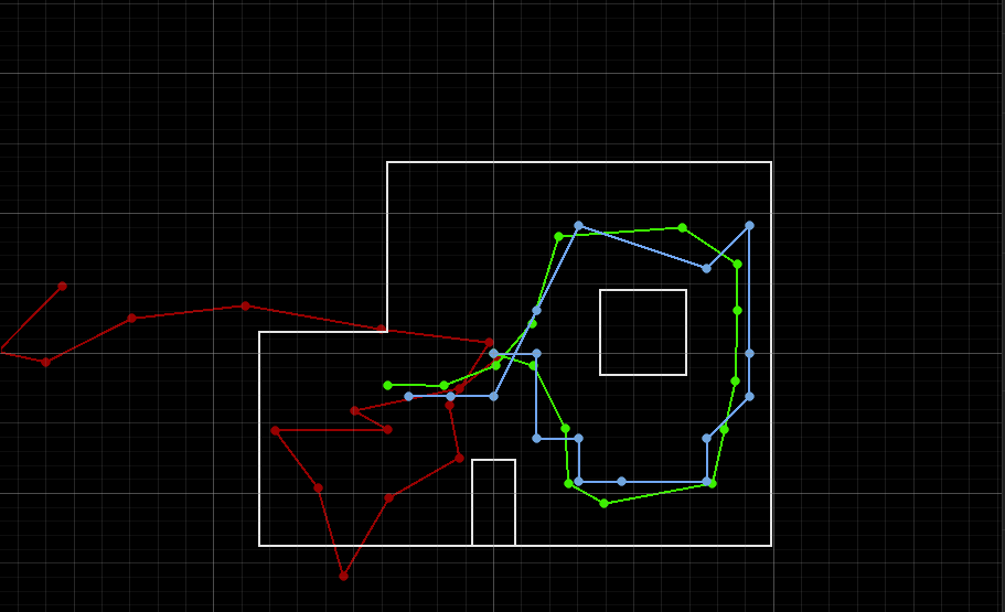
Now that the Bayes Filter has been implemented, I ran a simulation using the provided source code to model the robot's estimated position throughout a given trajectory. In the video below, three plots are shown. In green is the robot's ground truth position. This represents the robot's ideal position and orientation. In blue is the output of the Bayes Filter, representing the robot's predicted pose values. Finally, in red, is a model that uses raw odometry data without any probablistic modeling to estimate the robot's position. It is clear that the Bayes filter performs much better -- especially near walls, where the TOF sensor data is more accurate -- compared to the odoemetry model.
Acknowledgements
I referenced Stephan Wagner's and Daria Kot's 2024 Webpages while completing this lab.