Lab 11 - Performing Localization with the Physical Robot

In this lab, I expanded on the concepts developed in Lab 10. Previously, I had used a simulation of the robot to explore localization using a Bayes Filter. This algorithm combines the robot's prior belief about its location along with observations from its sensors to predict where it currently is within its known environment. While simulating this procedure proved to be a good first step, it was now time to implement this functionality on my physical robot.

Simulation

Before performing localization on the physical robot, I performed a simulation one more time, using optimized code provided by the course staff.

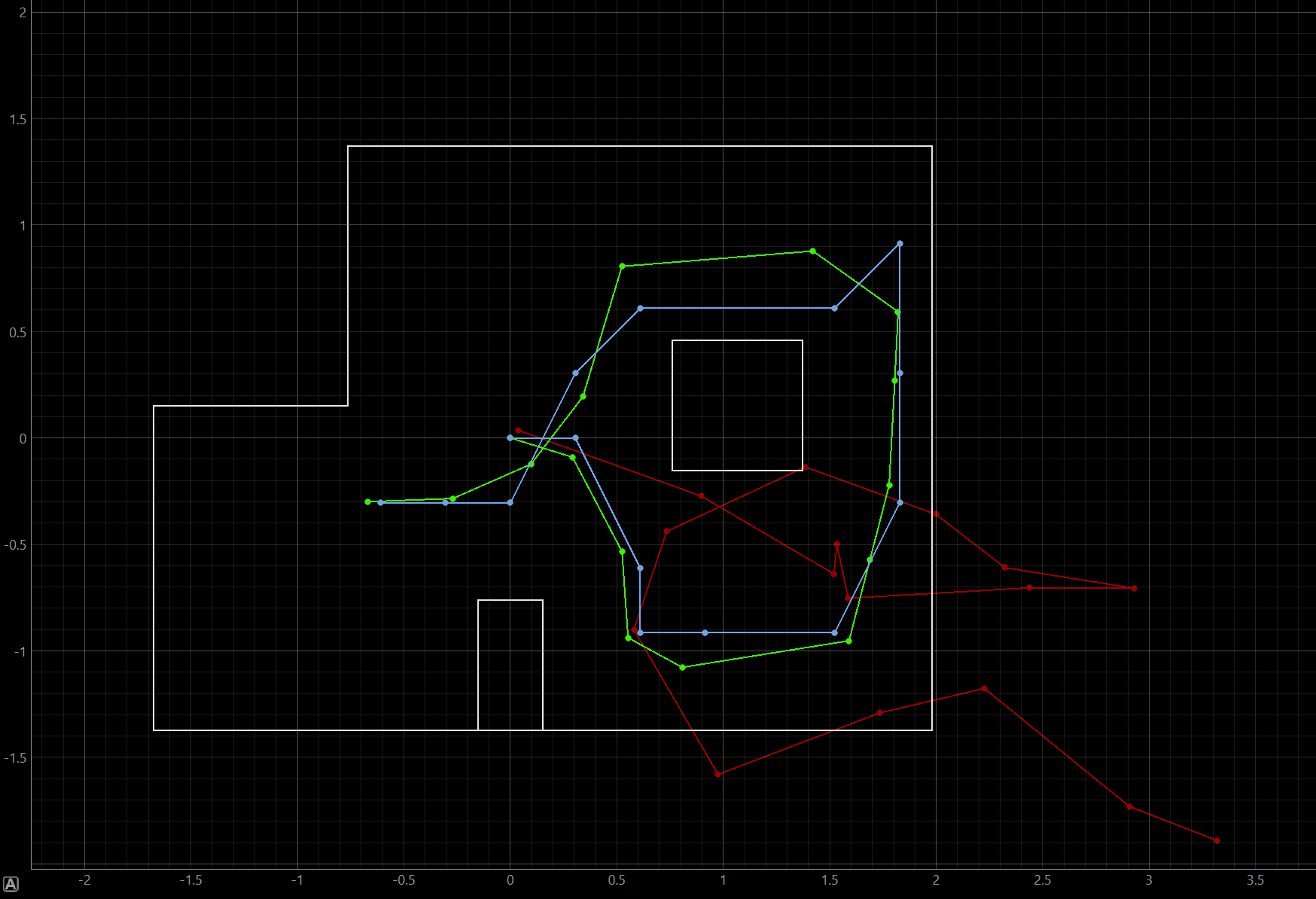
Shown above is a plot depicting the results of this simulation. The simulation uses the same map that is physically located in the lab space. During the simulation, the robot performs a simple trajectory, moving in an oval shape around a walled-off obstacle. The exact path that the robot takes is shown in green.

If we were to use odometry to determine the robot's position as it moves along this trajectory, we would fail miserably. Shown in red is the predicted location of the robot using odometry data. As seen in the graph, this localization technique performs quite poorly, as it shows that the robot moved through multiple walls and left its enclosed environment. This is not physically possible.

Luckily, the Bayes Filter provides us with a better estimate of the robot's current position. Shown in blue is the predicted location of the robot at each step on its trajectory, calculated using the Bayes Filter. Clearly, this algorithm performs MUCH better than simple odometry. At each time step, the robot tries to predict its location based on its prior beliefs about its pose. Then, the robot performs a 360 degree turn in 20 degree increments, recording TOF sensor data at each angle. Finally, the robot uses the sensor data along with its prior belief to update its current belief about where it is located. The Bayes Filter performs quite well as a method for robot localization.

Physical Implementation

Coincidentally, my robot's observation loop procedure from Lab 9 also performed 18 rotations in 20 degree increments, so I did not have to change too much on the Arduino side of my software. However, I made a few adjustments to my on-robot code to better suit the needs of this lab.

First, I updated my sensor data recording function. In lab 9, I had my robot record 5 data points from each front-facing TOF sensor at each angle location. Then, I recorded each of these measurements separately to array indicies. This resulted in a total of 180 data points (2 Sensors * 5 Data Points / Rotation * 18 Rotations) being transmitted for each observation loop. However, the Bayes Filter Python code works only by using column vectors of length 18. I decided to account for this on the Arduino side rather than the Python side. I updated my code to record the mean value of all of its sensor measurements at each angle, resulting in 1 recorded TOF value for each angle. In total, this resulted in my robot only transmitting 18 data points per observation loop rather than 180. Shown below is my updated code:

void RECORD_MAP(){
  measure_DMP_data();
  dist_mean = 0;
  yaw_mean = 0;
  for(int i = 0; i < 5; i++){
    distanceSensor1.startRanging();
    distanceSensor2.startRanging();
    while(!distanceSensor1.checkForDataReady()){

    }
    while(!distanceSensor2.checkForDataReady()){
      
    }
    dist_mean += distanceSensor1.getDistance();
    dist_mean += distanceSensor2.getDistance();
    yaw_mean += DMP_YAW;
    distanceSensor1.clearInterrupt();
    distanceSensor2.clearInterrupt();
  }
  distanceSensor1.stopRanging();
  distanceSensor2.stopRanging();
  dist_mean = dist_mean / 10;
  yaw_mean = yaw_mean / 5;

  tof1_stamps[INDEX] = dist_mean;
  yaw_array[INDEX] = yaw_mean;
  INDEX += 1;
}

I also updated my observation loop code to only transmit two data arrays rather than three, as all of the TOF sensor data was now fit into a single array:

for(int i = 0; i < INDEX; i++){
    tx_estring_value.clear();
    tx_estring_value.append(tof1_stamps[i]);
    tx_estring_value.append("|");
    tx_estring_value.append(yaw_array[i]);
    tx_characteristic_string.writeValue(tx_estring_value.c_str());
}

On the Python side, things were a bit more tricky, but not too complicated. However, I did run into an issue using the Lab 11 Jupyter Notebook. When I tried to connect via Bluetooth to the Artemis, the notebook produced a ridiculously long error. Luckily, there was an Ed Discussion post about this exact error and how to fix it, so this only set me back a few hours - uninstalling Anaconda and restarting my laptop took a lot longer than I expected and caused my laptop to update to Windows 11 :(

Since my observation loop BLE command performs both the physical rotation and the data communication process within the same command, my Python code was not too difficult to implement. I created a notification handler to process the incoming data - both Yaw and TOF distance measurements. I also knew that when the robot's data had finished being transmitted, it should be stored in an 18-length array on the Python side. So, I used the asynchronous sleep command as outlined in the lab handout. Once the Python controller sends the "START OBSERVATION LOOP" command to the robot, the Python code enters a while loop and "sleeps" until it detects that the data arrays have 18 entries in them. Finally, I convert the data arrays into the correct format - column vectors - and return them, ending the observation loop function and allowing the Bayes Filter to continue its update step. Shown below is my implementation in Python:

def perform_observation_loop(self, rot_vel=120):
        """Perform the observation loop behavior on the real robot, where the robot does  
        a 360 degree turn in place while collecting equidistant (in the angular space) sensor
        readings, with the first sensor reading taken at the robot's current heading. 
        The number of sensor readings depends on "observations_count"(=18) defined in world.yaml.
        
        Keyword arguments:
            rot_vel -- (Optional) Angular Velocity for loop (degrees/second)
                        Do not remove this parameter from the function definition, even if you don't use it.
        Returns:
            sensor_ranges   -- A column numpy array of the range values (meters)
            sensor_bearings -- A column numpy array of the bearings at which the sensor readings were taken (degrees)
                               The bearing values are not used in the Localization module, so you may return a empty numpy array
        """
        sensor_ranges = []
        sensor_bearings = []

        def lab11_handler(uuid, value):
            raw_value = ble.bytearray_to_string(value)
            data = raw_value.split('|')
            sensor_ranges.append(float(data[0]) / 1000)
            sensor_bearings.append(float(data[1]))

        async def sleep_for_three_seconds():
            await asyncio.sleep(3)
        
        ble.start_notify(ble.uuid['RX_STRING'], lab11_handler);
        ble.send_command(CMD.LAB_11_LOOP,"")
        
        while(len(sensor_ranges) < 18):
            await sleep_for_three_seconds()

        ble.stop_notify(ble.uuid['RX_STRING'])

        sensor_ranges = np.array(sensor_ranges)[np.newaxis].T
        sensor_bearings = np.array(sensor_bearings)[np.newaxis].T

        return sensor_ranges, sensor_bearings

Testing and Results

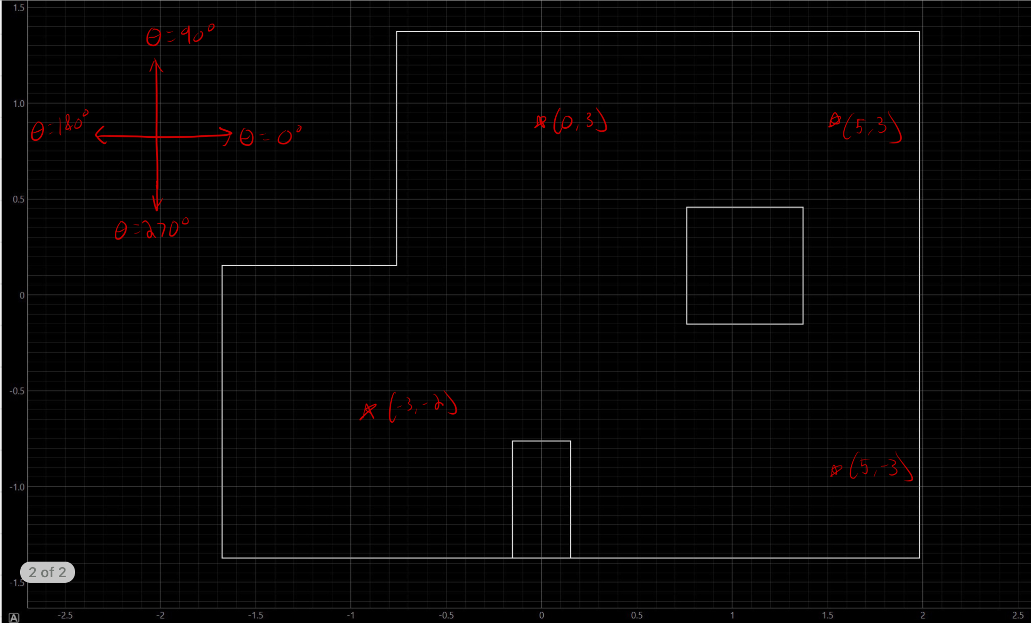
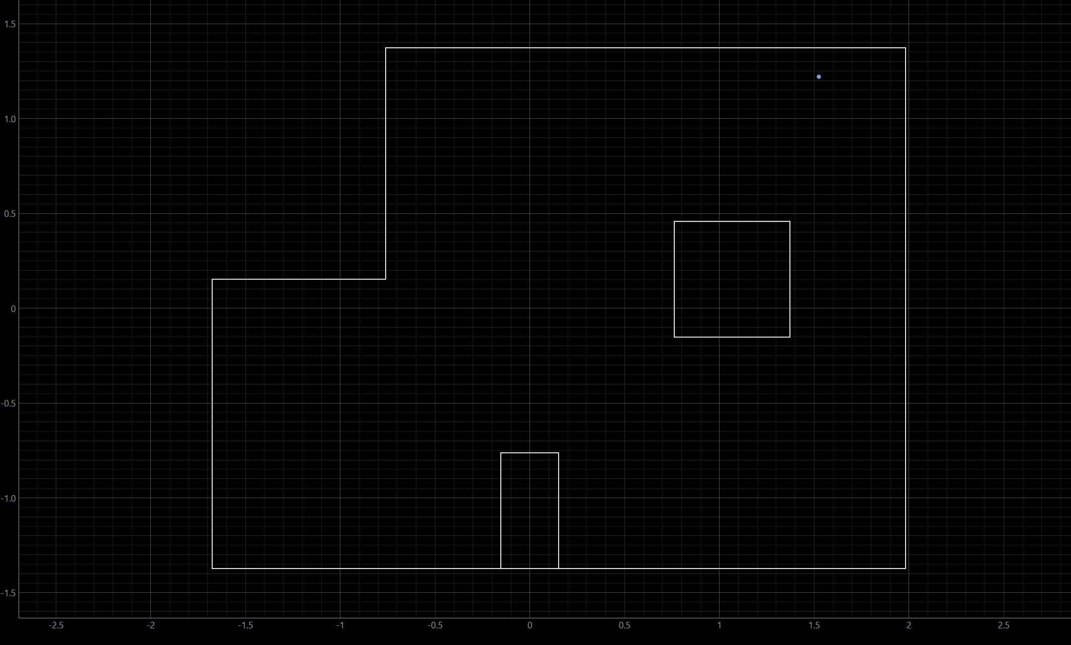
Now that my software had been updated, it was time to perform localization in the real world! This was performed using the physical map space in the lab, which is the same shape as the map in the previously shown simulations. As I did not perform Lab 9 using this map space, it was exciting to finally use it for this lab! Since the mechanics/physical execution of observation loop had already been finely tuned during my lab 9 efforts, updating the software was relatively straightforward and I was able to quickly begin on testing my robot's performance. Shown below are the four map locations that I tested the robot at, followed by the Bayes Filter's prediction for each test.

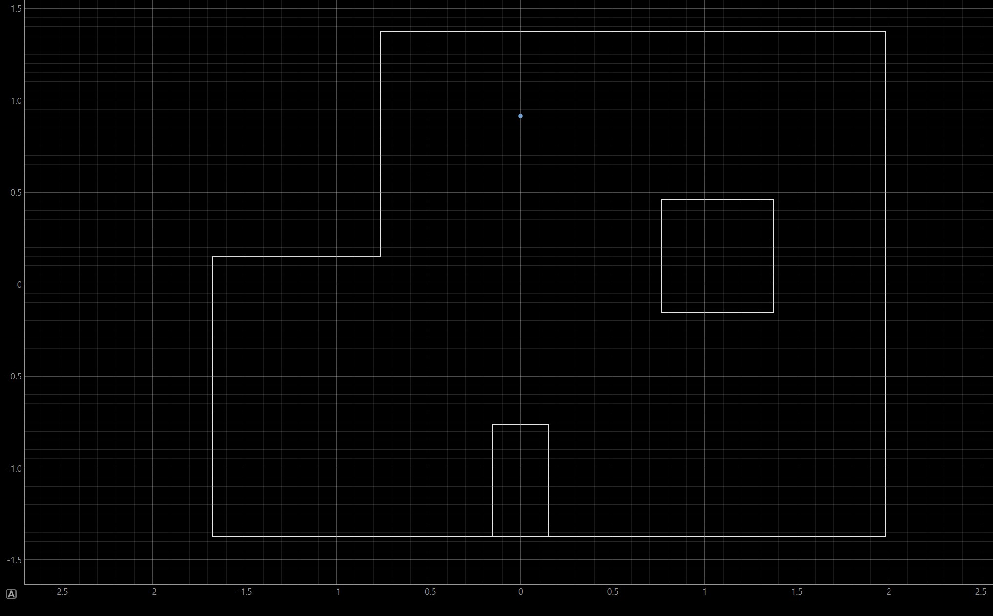
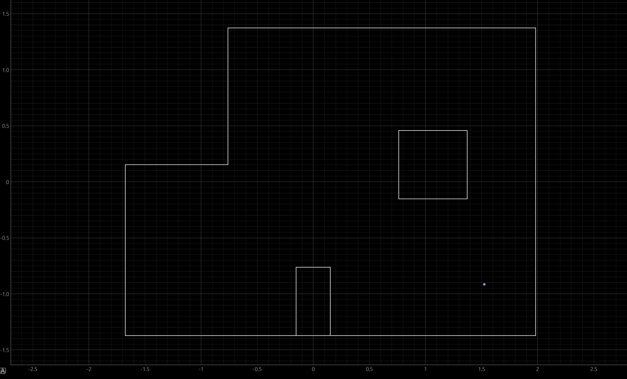
As seen in the maps above, my robot performed quite well. I believe that this is mainly due to my robot's precise movement as it performs each observation loop. During Lab 9, my robot initially experienced about 6 inches of drift when performing each loop. When the Bayes Filter executes, each possible location is discretized to reduce computation complexity (it would take infinite memory to map each continuous point in the map). This drift may have caused the robot's belief to be quite inaccurate. Each discretized box is 1 foot by 1 foot, so having 6 inches of drift could push the robot to believe it's in a much different location.

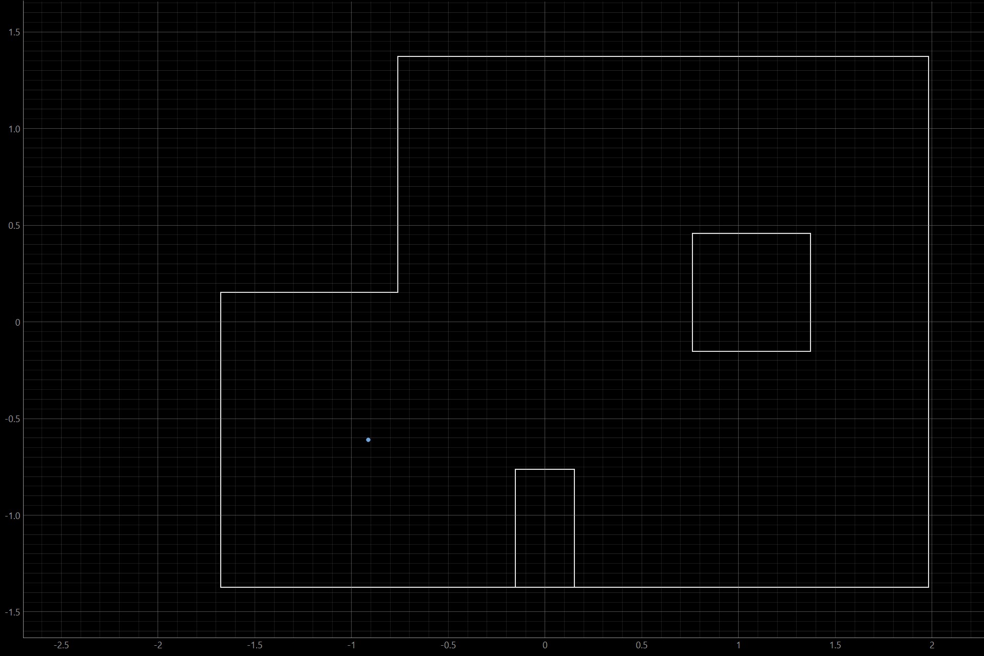
However, I worked hard to perfect my observation loop mechanics, and my robot experiences close to zero drift when it performs each loop (see lab 9 for video example). Therefore, it makes sense that my robot's predicted locations are quite accurate when compared to their real life ground truths.

In fact, the only location that the Bayes Filter estimated inaccurately was the spot at (5,3). The Bayes Filter predicted that the robot was at location (5,4). However, this is only 1 foot off from its actual location, and the Bayes Filter performed exceptionally well for the other locations. Therefore, I believe that it is safe to say that my robot performs localization quite well.

Overall, this lab was quite satisfying to complete. I enjoyed seeing my robot perform more sophisticated tasks, combining parts of previous labs. I am excited to implement path planning and complete my robot with next week's lab!

Acknowledgement

I consulted Nila Narayan's and Stephan Wagner's Lab 11 webpages while completing this lab.