Table of Contents
Setup
This lab focuses on the IMU sensor that will be incorporated into my robot. The IMU contains three sensors - an accelerometer, a gyroscope, and a magnetometer.
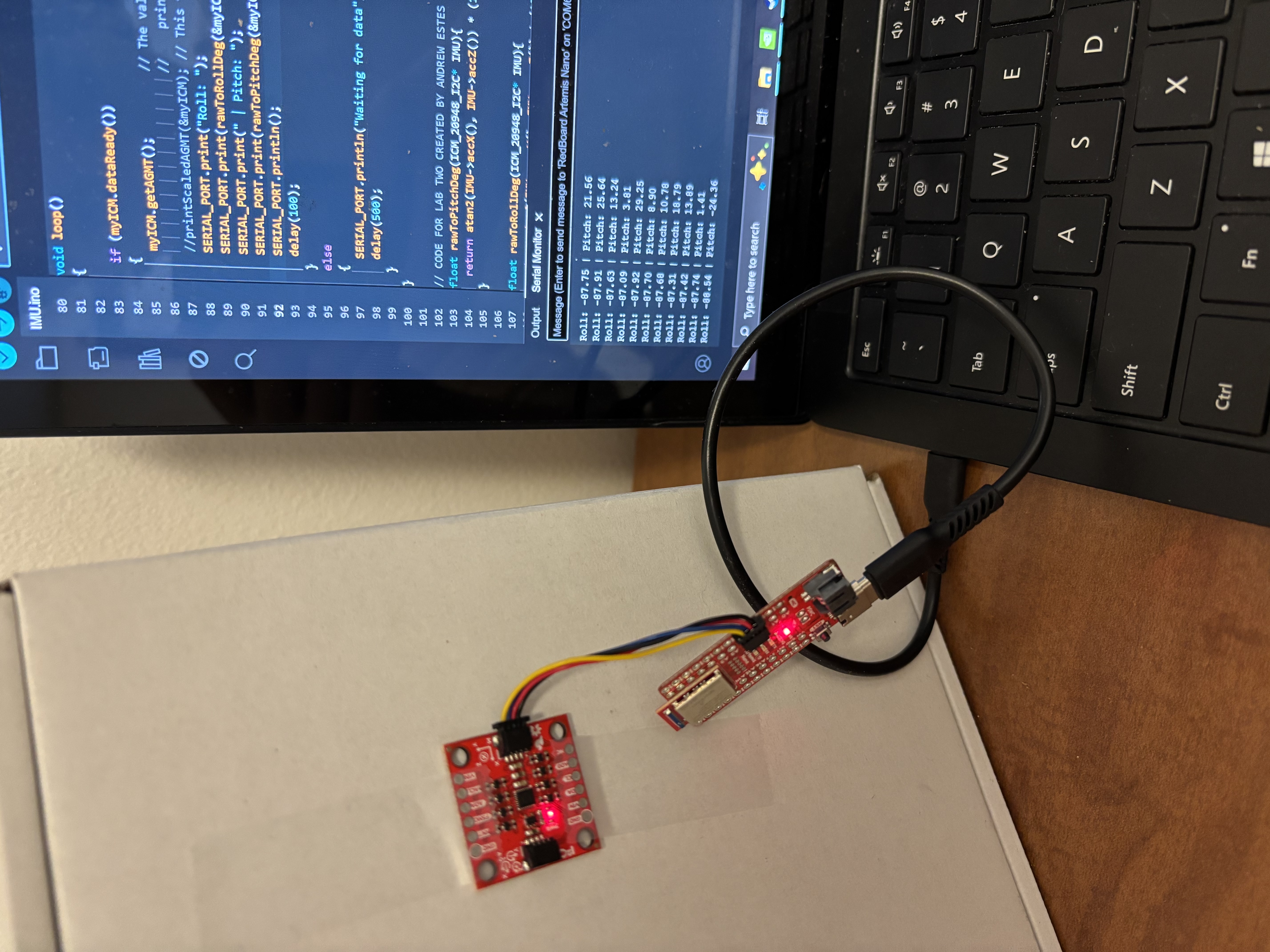
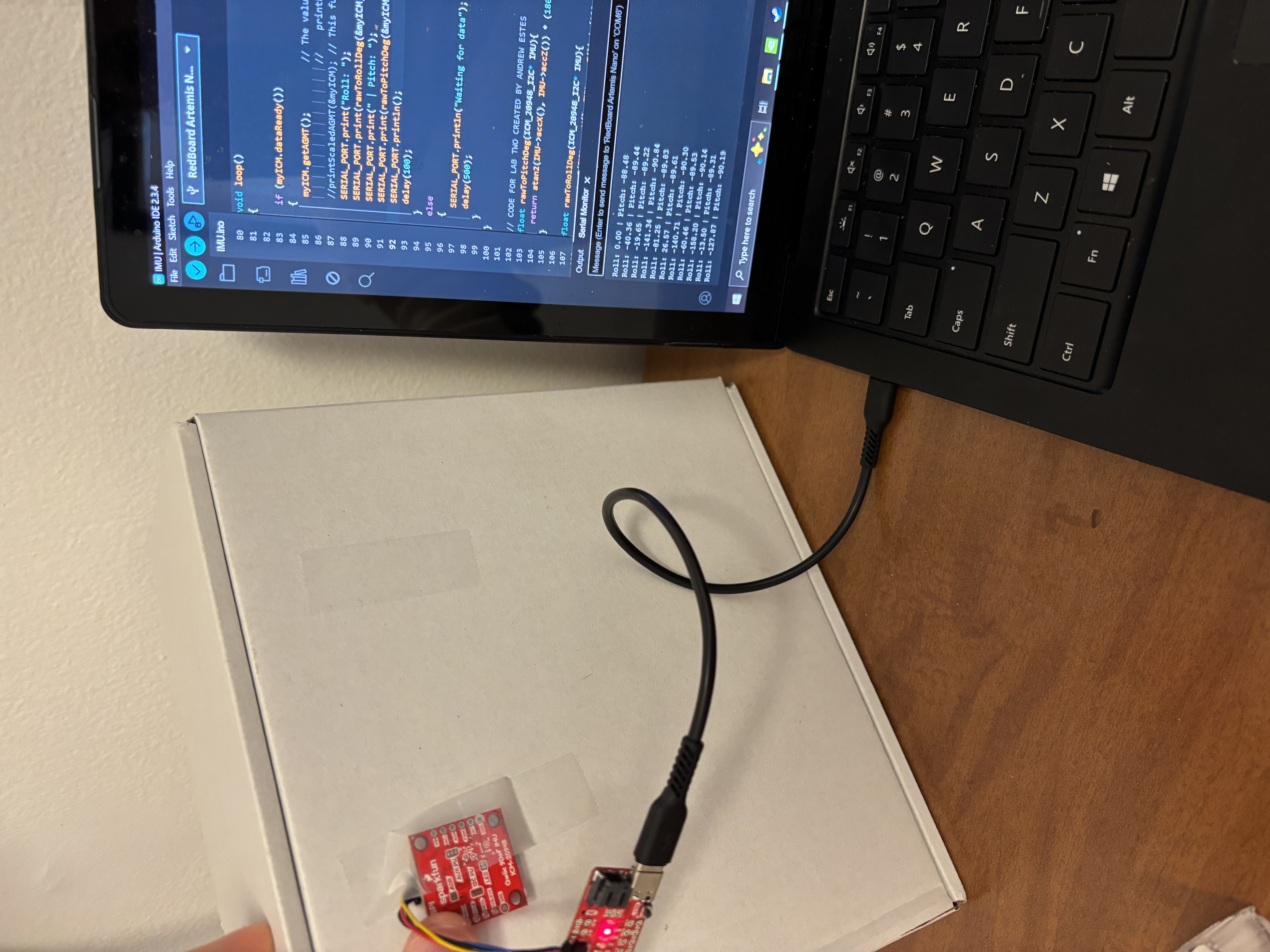
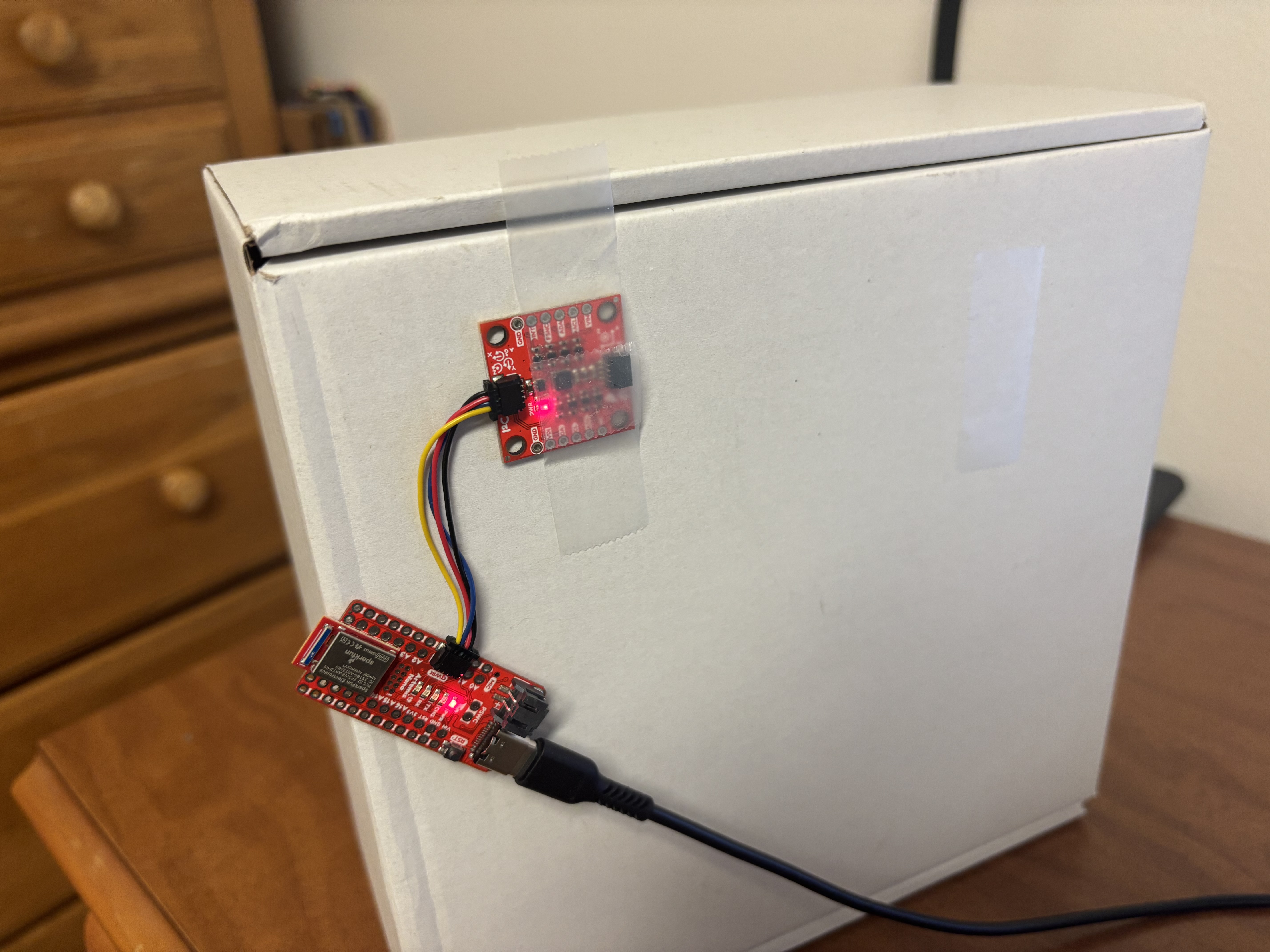
To begin, I used a QWIIC cable to connect the IMU to the Artemis as seen below:
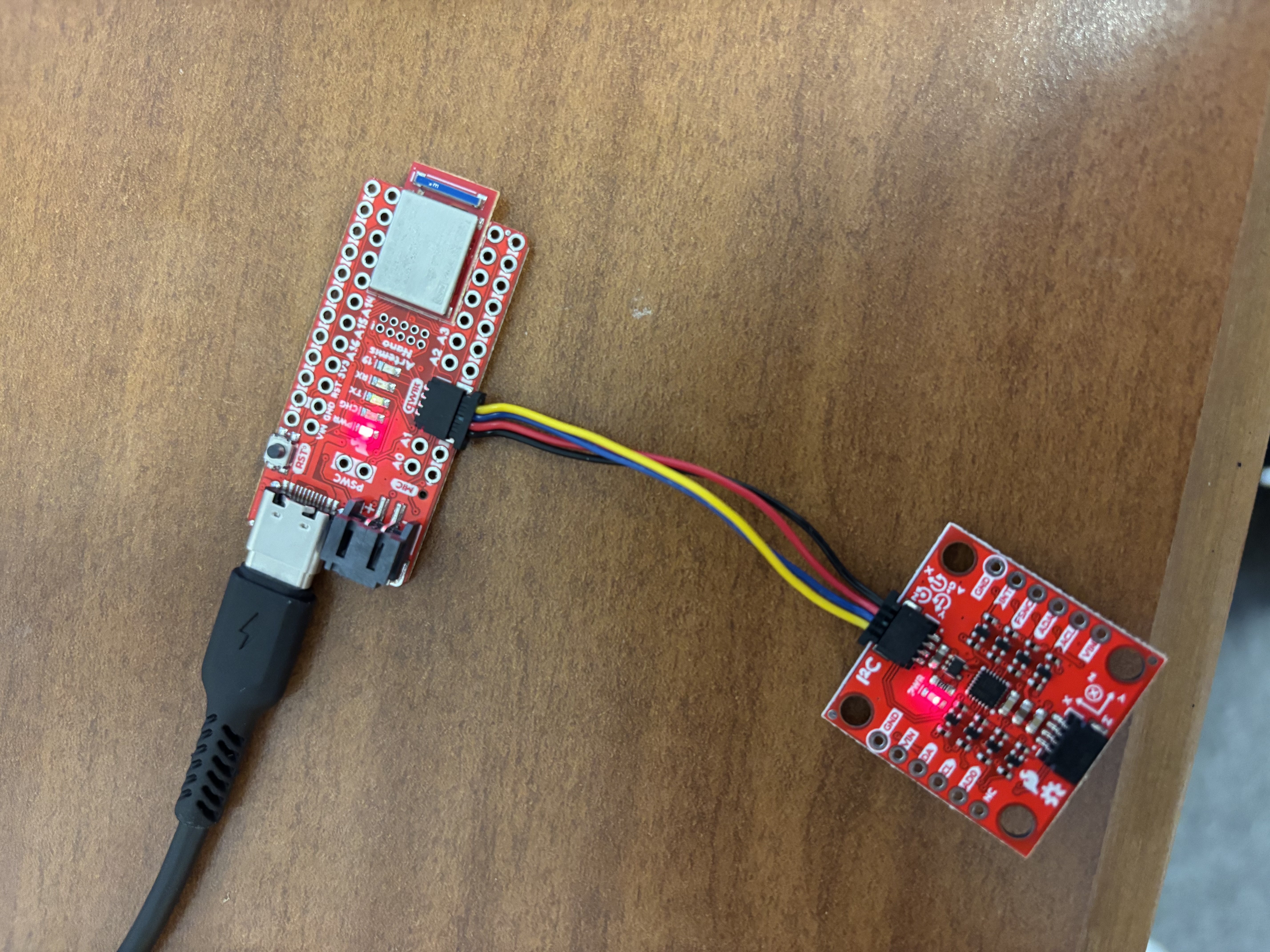
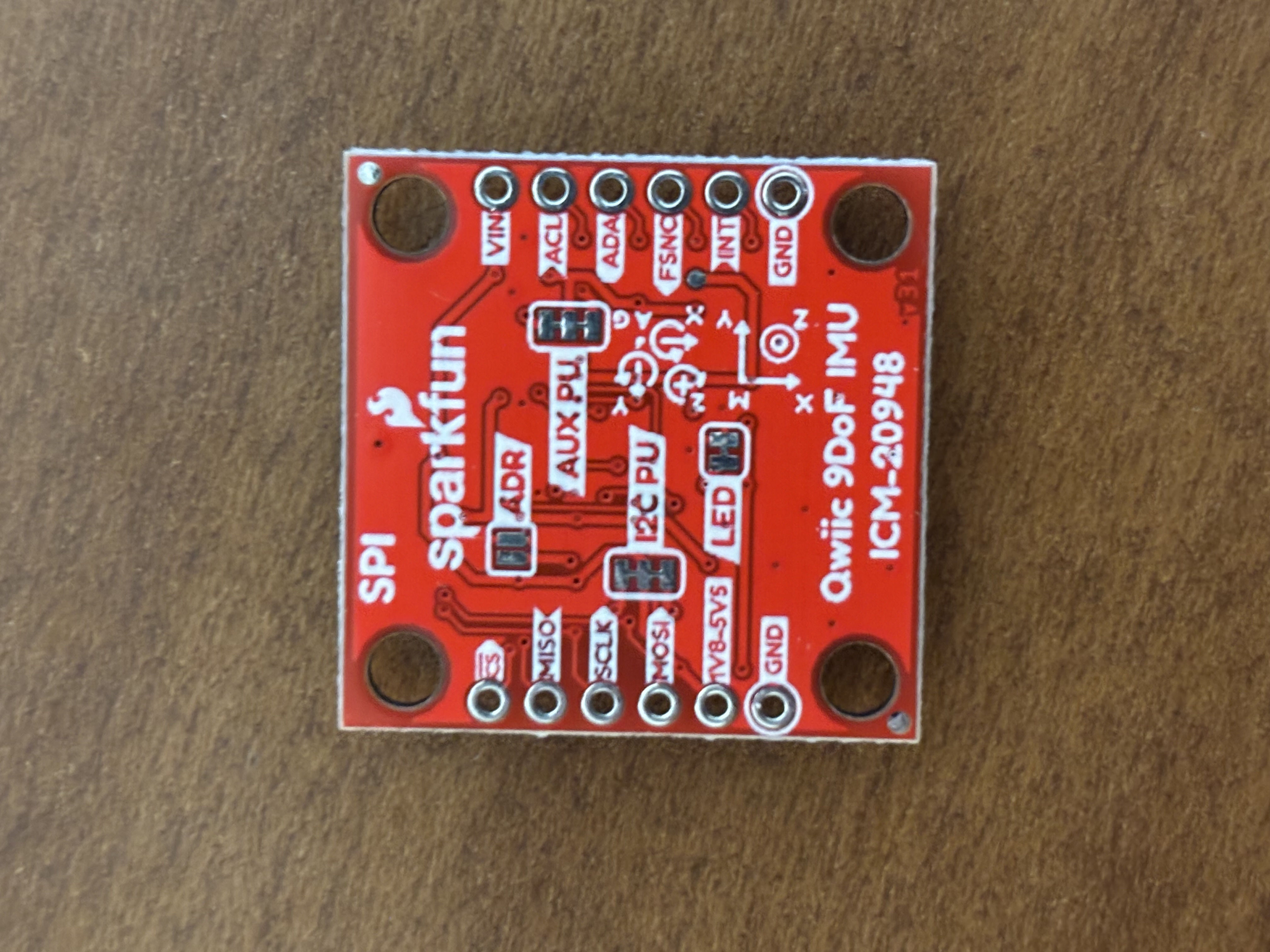
Now that I had the IMU connected to the Artemis, I had to check which value to assign to the AD0_VAL macro. Since the ADR jumper on the IMU board is open, I assigned a value of 1 to AD0_VAL, as instructed by the comments provided in the Arduino example code.
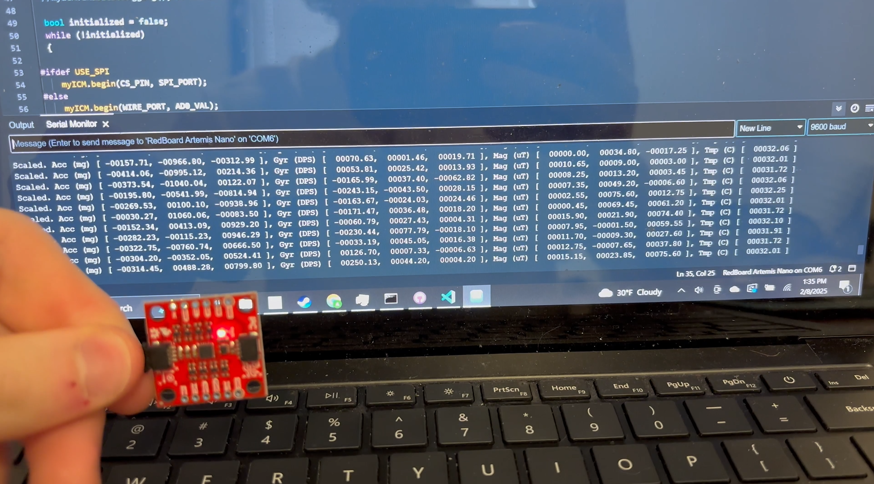
Next, I ran the example IMU code in order to test that my sensor was properly recording data. As seen in the video below, when the IMU is accelerated lineraly, the corresponding accelerometer values printed to the Serial Monitor will change. Similarly, when the IMU is rotated, the corresponding gyroscope values will change.
Accelerometer Test
In this video, the IMU is linerally accelerated in the X(Pink), Y(Blue), and Z(Yellow) direction. When the board is accelerated in a specific direction, you can see the corresponding plotted curve react to the motion.

Gyroscope Test
Next, I tested the gyroscope using the example code. As seen in the video below, when the IMU is rotated, the gyroscope data values (recorded in degrees per second) are output to the serial monitor. When the IMU is stationary, these values float around zero (with some flucuation due to noise). When the IMU is rotated, these values increase significantly, indicating that the sensor is abel to accurately record a change in rotation.
Blue LED Indicator
The last part of my setup involved blinking the Artemis' onboard LED after the IMU sensor had been properly initialized. This helps with debugging and allows the user to determine if the sensor is setup correctly. This was accomplished by adding a few lines of code to the setup() function in my Arduino program.
  pinMode(LED_BUILTIN, OUTPUT);
  for(int i = 0; i < 3; i++){
    digitalWrite(LED_BUILTIN, HIGH);
    delay(500);
    digitalWrite(LED_BUILTIN, LOW);
    delay(500);
  }
Accelerometer
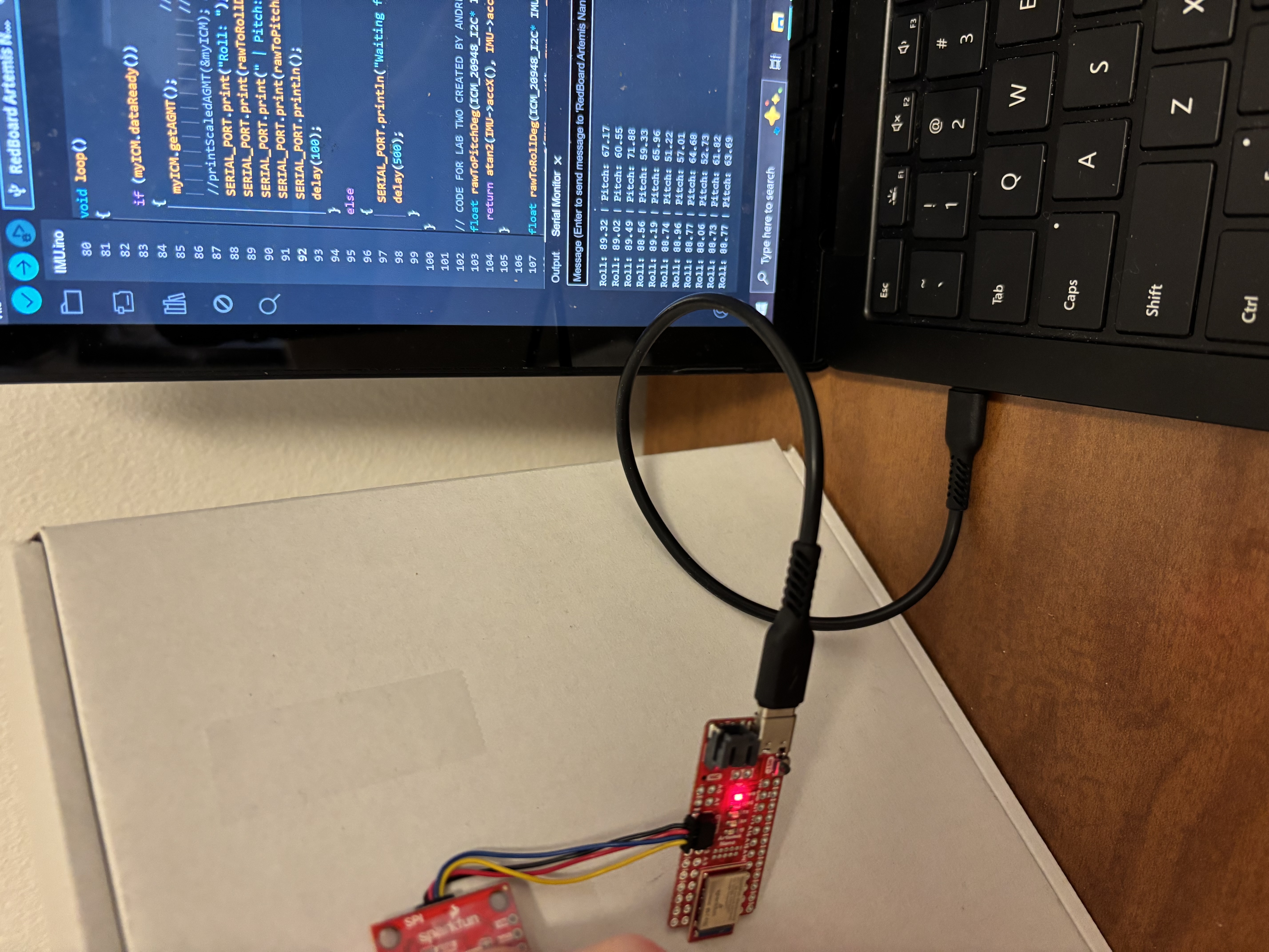
To begin working with the accelerometer, I implemented two functions that converted the raw acceleration data into roll and pitch quantities. I used the C math library's atan2() function to compute these values correctly. I also implemented two point calibration within these functions. While the accelerometer is relatively accurate, there was some error in its recordings prior to calibration. For example, when holding the IMU board directly against a wall, the readings were slightly off from the expected value of 90 degrees. For this reason, I implemented calibration.
Seen below is the output of the accelerometer's roll and pitch recordings prior to implementing calibration:
90 Degrees Roll
-90 Degrees Roll
90 Degrees Pitch

-90 Degrees Pitch
float correctedPitchDeg(ICM_20948_I2C* IMU){
  float refLow = -90.0;
  float refHigh = 90.0;
  float rawLow = -88.54;
  float rawHigh = 88.77;
  float refRange = refHigh - refLow;
  float rawRange = rawHigh - rawLow;
  float measure = atan2(IMU->accX(), IMU->accZ()) * (180 / M_PI);
  float correct = (((measure - rawLow) * refRange) / rawRange ) + refLow;
  return correct;
}

float correctedRollDeg(ICM_20948_I2C* IMU){
  float refLow = -90.0;
  float refHigh = 90.0;
  float rawLow = -90.19;
  float rawHigh = 87.96;
  float refRange = refHigh - refLow;
  float rawRange = rawHigh - rawLow;
  float measure = atan2(IMU->accY(), IMU->accZ()) * (180 / M_PI);
  float correct = (((measure - rawLow) * refRange) / rawRange ) + refLow;
  return correct;
}
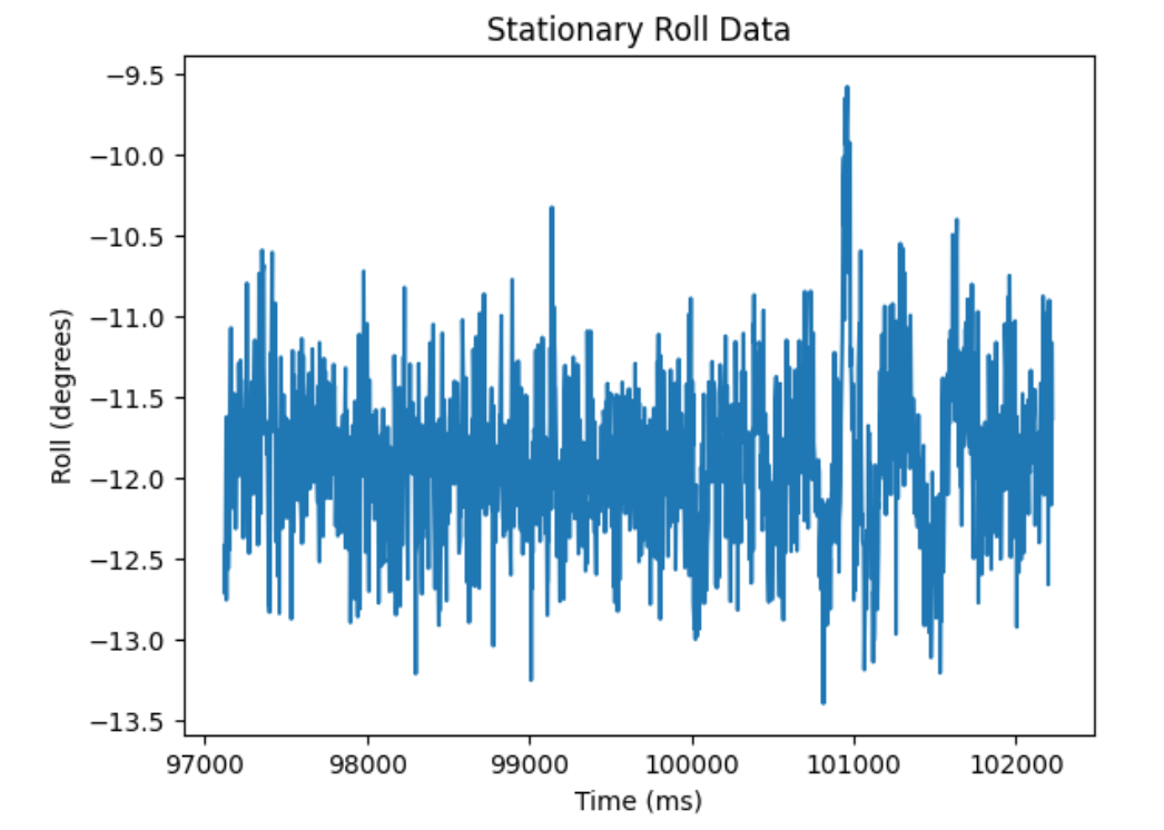
While this calibration scheme helped improve the accuracy of the accelerometer, the recorded data was still quite noisy. To reduce the sensor's noise, I began by analyzing the frequency spectrum of the sensor's roll and pitch data. I collected four sets of data: stationary and moving data for both the roll and pitch measurements. When taking measurements, I determined that I could record 1587 datapoints in 5.098 seconds, resulting in a sample rate of 311 samples per second.
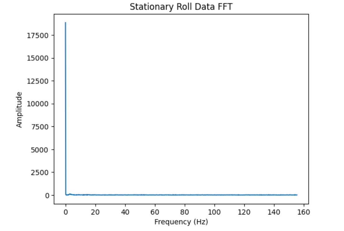
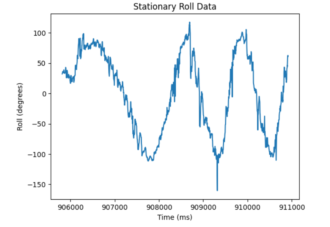
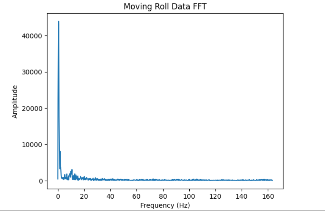
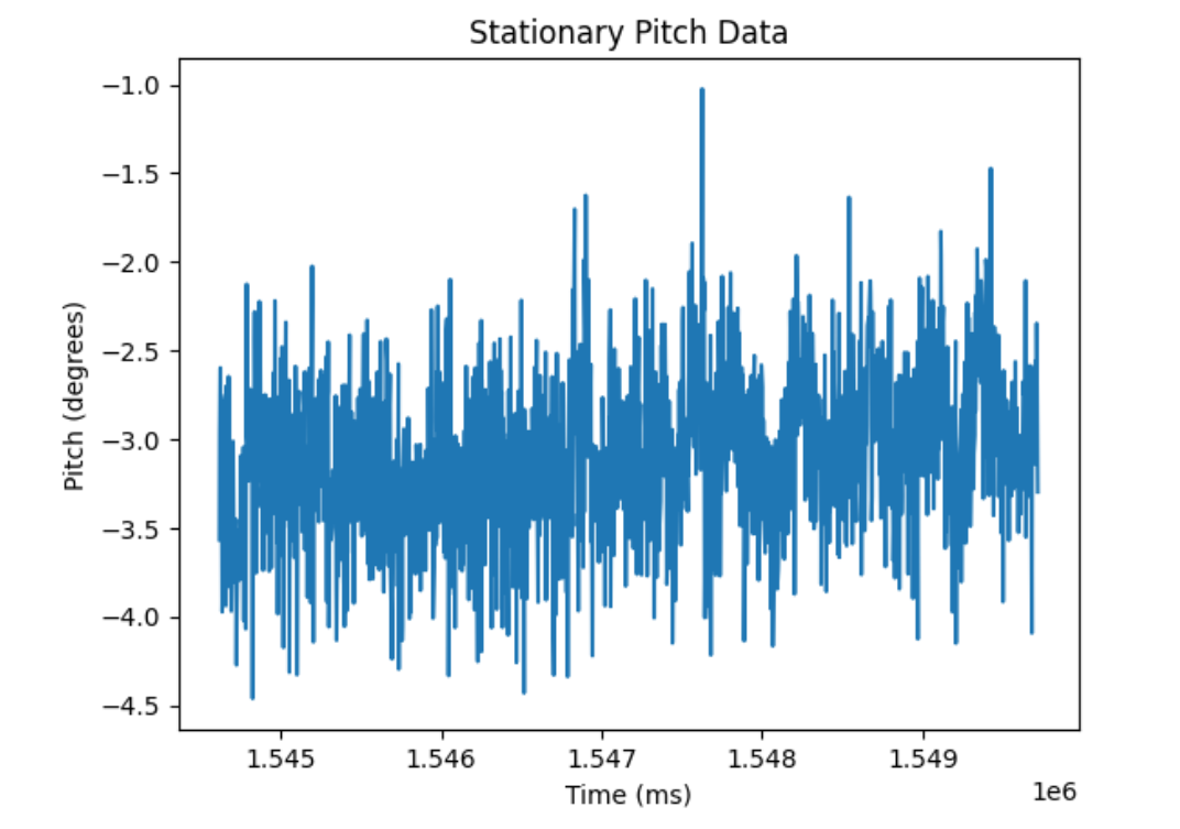
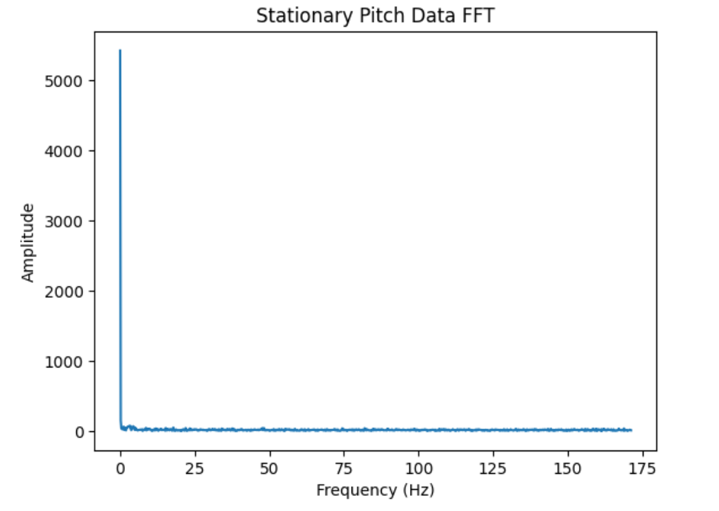
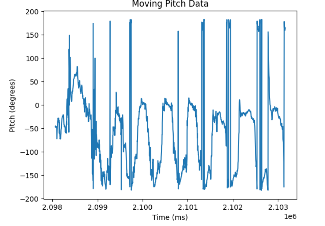
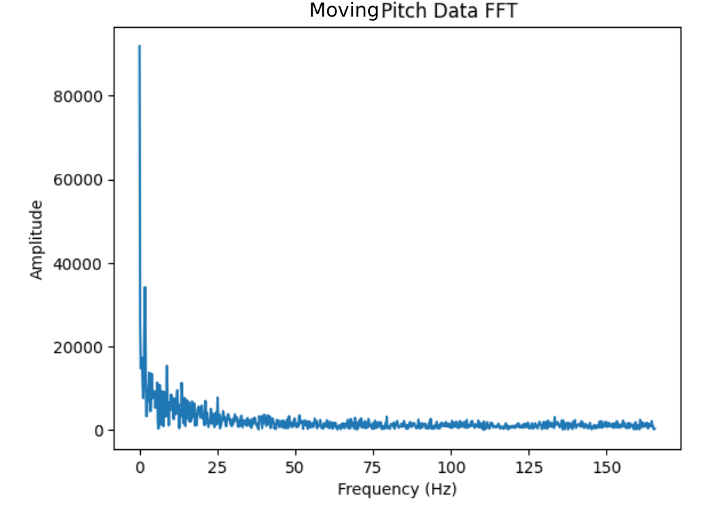
By analyzing each plot, it is clear that most of the significant frequency content is contained below 5 Hz. With the stationary recordings, nearly all of the frequency content is at 0 Hz. With the moving recordings, higher frequencies are detected at significant amplitudes, but this is likely due to the sensor's angle reading switching rapidly between -180 and 180 degrees, as seen in the Moving Pitch graph. With this analysis complete, I implemented a low-pass filter with a cutoff frequency of 2 Hz.
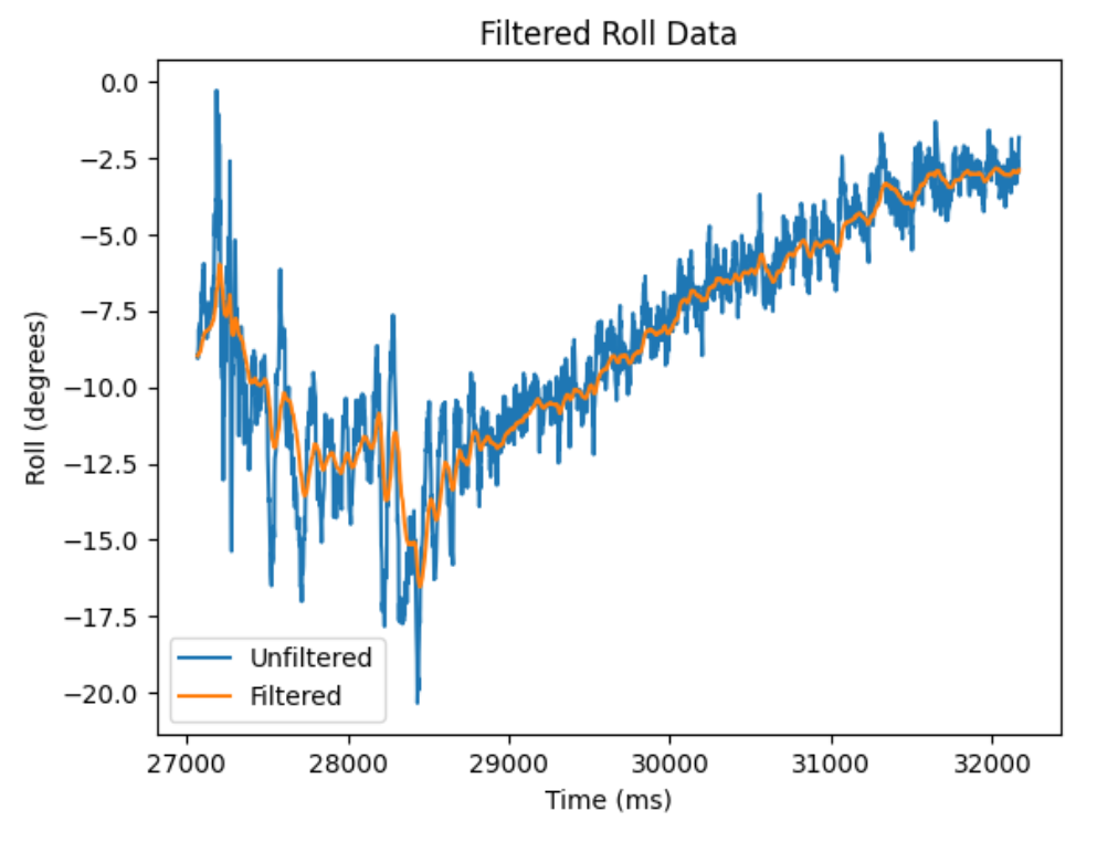
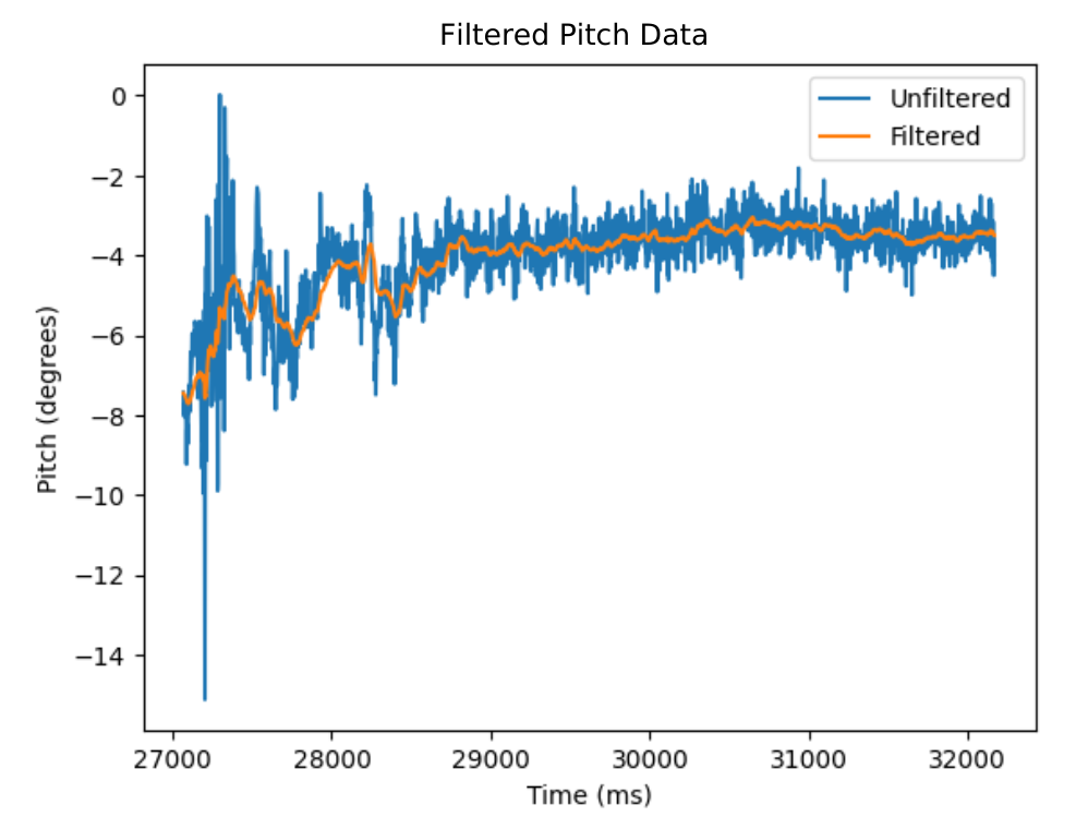
Using a sample rate of 311 samples per second and a cutoff frequency of 2 Hz, I calculated my filter's alpha value to be 0.0388. Seen in the graphs below, this filter drastically reduced the amount of noise present in the sensor's measurements.
Gyroscope
To begin testing my gyroscope, I implemented a bluetooth command that would correctly convert the raw gyroscope measurements into roll, pitch, and yaw, as seen below:
int start_time = (int)millis();
int index = 1;
float lastTime = millis();
time_stamps[0] = millis();
gyro_roll[0] = 0;
gyro_pitch[0] = 0;
gyro_yaw[0] = 0;
// Record Time Data Rapidly
while((int)millis() < start_time + RECORD_TIME && index < TIME_ARRAY_SIZE){
  if (myICM.dataReady()){
    myICM.getAGMT(); // Collect data for RECORD_TIME ms
    time_stamps[index] = (int)millis();
    float dt = (millis() - lastTime) / 1000;
    lastTime = millis();
    gyro_roll[index] = gyro_roll[index - 1] + myICM.gyrX()*dt;
    gyro_pitch[index] = gyro_pitch[index - 1] + myICM.gyrY()*dt;
    gyro_yaw[index] = gyro_yaw[index - 1] + myICM.gyrZ()*dt;
    index++;
  }
}
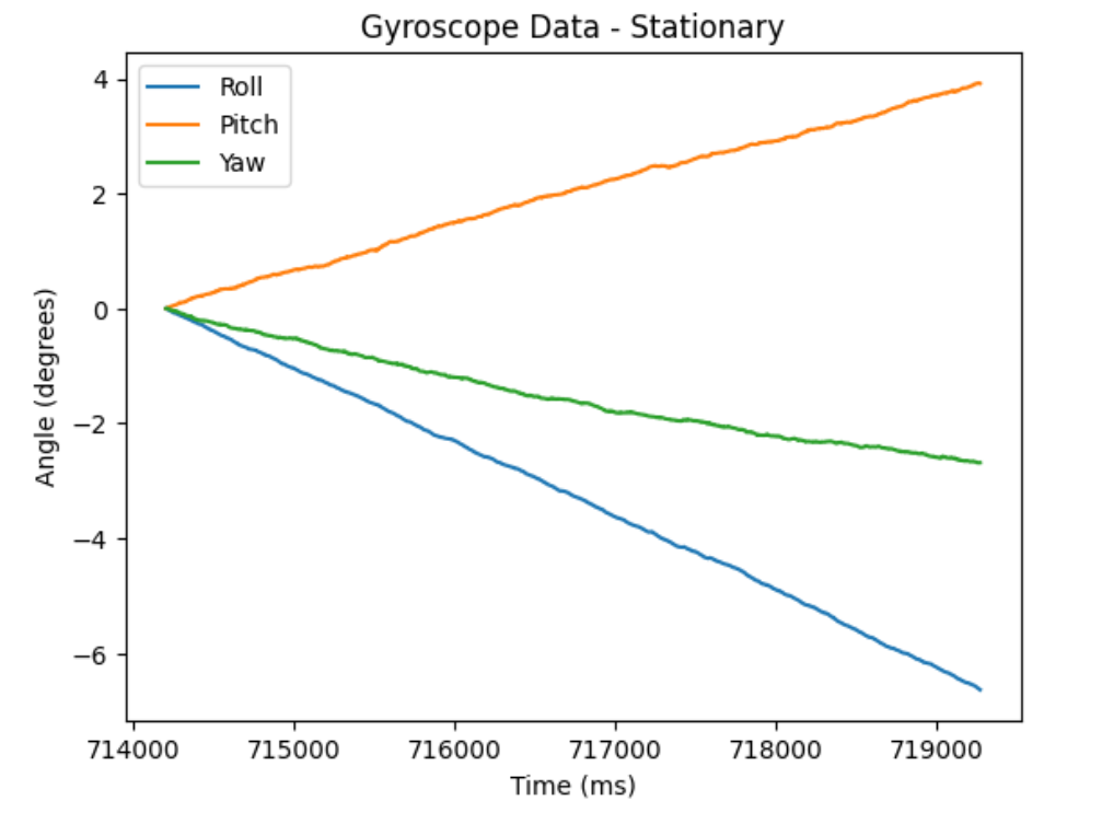
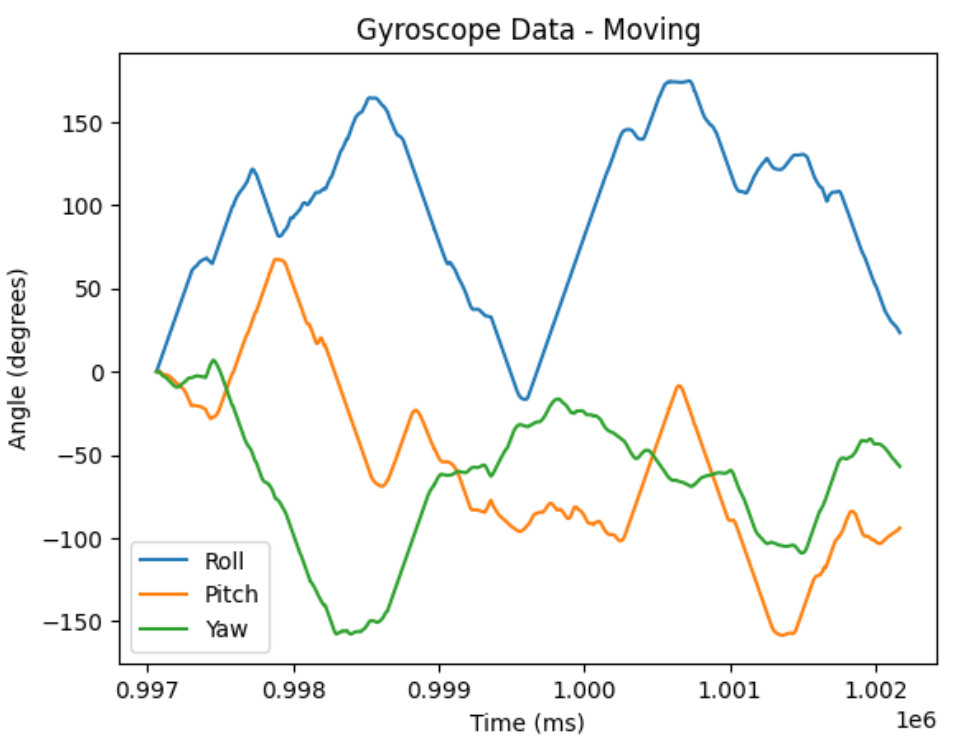
When testing my gyroscope in a stationary position, I noticed that there was a large amount of drift in the sensor's readings. When the sensor was moving, the readings proved to be more accurate. While the gyroscope is less noisy than the accelerometer, the accelerometer was not as susceptible to drift, so I needed to incorporate a filter that combined the data from each sensor.
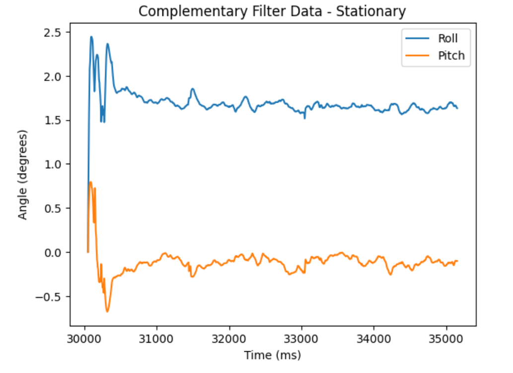
To create my filter, I weighted the gyroscope data with a bias of 0.9, and the accelerometer data was weighted with a bias of 0.1. I chose these values because the gyroscope proved to be far more accurate and less noisy than the accelerometer, but needed data to counter the drift effect of the gyroscope. This filter was applied to the IMU's roll and pitch measurements. Since the accelerometer is not able to measure yaw, I did not apply this filter to the yaw measurement.
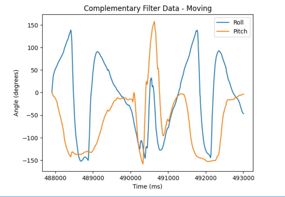
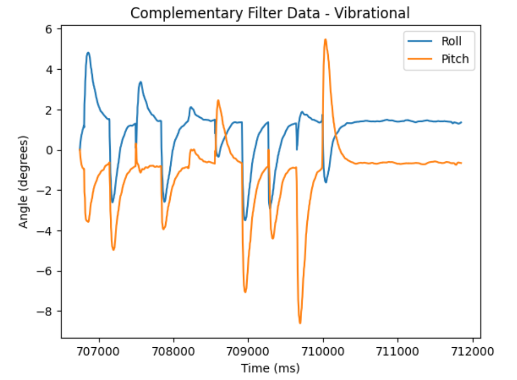
With this filter applied, I was able to record both roll and pitch measurements with high accuracy, low noise, and low drift. I conducted three tests - stationary, moving, and vibrational - and the results are shown below. When the IMU is stationary, it is resistant to noise and drift. When the IMU is moving, it is almost free of noise. When the IMU experiences vibrations, it is able to quickly return to recording accruate measurements.
Sampling Data
Now that all of my tests were complete, it was time to speed up the rate at which I could record IMU data. I removed all calls to the delay() function and removed all print statements from my IMU measurement command. After recording data, I measured that I collected 1782 samples in 5.098 seconds. This corresponds to a sampling rate of roughly 349 samples per second. I recorded data in separate arrays in order to facilitate the transmission of data over Bluetooth. If I were to use one large array, it would be extremely difficult to parse and find specific pieces of data. Likewise, since an array can only hold one type of data, this would make organization even more difficult. For this reason, I chose to create seperate arrays for each measurement type. As of now, I have ten distinct arrays for holding raw or filtered accelerometer and gyroscope data. I stored my time data as integers, since precision to the nearest millisecond has proved sufficient so far. I have recorded all of my other data measurements as floats, since these values can and likely will hold noninteger values in reality. With 1782 data points per array being sampled in a time of roughly 5 seconds, and ten arrays being used, this results in 17820 data points in 5.098 seconds, or 3495 data points per second. If each data point is 4 bytes, this results in the Artemis' memory being filled at a rate of 13.98 kilobytes per second. As seen in most of the graphs in this report, the time scale spans just over 5 seconds, proving that my Artemis is capable of recording at least 5 seconds of data and transmitting it over Bluetooth. Attached below is my code for transmitting the complementary filter data via Bluetooth:
case COMP_FILTER_IMU:{
    int start_time = (int)millis();
    int index = 0;
    float lastTime = millis();
    time_stamps[0] = millis();
    gyro_roll[0] = 0;
    gyro_pitch[0] = 0;
    // Record Time Data Rapidly
    while((int)millis() < start_time + RECORD_TIME && index < TIME_ARRAY_SIZE){
      if (myICM.dataReady()){
        myICM.getAGMT(); // Collect data for RECORD_TIME ms
        time_stamps[index] = (int)millis();
        float dt = (millis() - lastTime) / 1000;
        lastTime = millis();
        gyro_roll[index] = gyro_roll[index - 1] + myICM.gyrX()*dt;
        gyro_pitch[index] = gyro_pitch[index - 1] + myICM.gyrY()*dt;
        roll_stamps[index] = correctedRollDeg(&myICM);
        pitch_stamps[index] =  correctedPitchDeg(&myICM);
        index++;
      }
    }
    // Begin Filtering
    float alpha = 0.0388;
    roll_filter_stamps[0] = roll_stamps[0];
    pitch_filter_stamps[0] = pitch_stamps[0];

    for(int i = 1; i < index; i++){
      roll_filter_stamps[i] = alpha*roll_stamps[i] + (1 - alpha)*roll_filter_stamps[i-1];
      roll_filter_stamps[i-1] = roll_filter_stamps[i];
      pitch_filter_stamps[i] = alpha*pitch_stamps[i] + (1 - alpha)*pitch_filter_stamps[i-1];
      pitch_filter_stamps[i-1] = pitch_filter_stamps[i];
      float dt = (millis() - lastTime) / 1000;
      lastTime = millis();
      comp_roll[i] = (comp_roll[i - 1] - gyro_roll[i]*dt)*0.9 + 0.1*roll_filter_stamps[i];
      comp_pitch[i] = (comp_pitch[i - 1] + gyro_pitch[i]*dt)*0.9 + 0.1*pitch_filter_stamps[i];
    }
    // Send Arrays of Data
    for(int i = 0; i < index; i++){ // If array does not fill in alloted time, only send recorded values and not empty indicies
      tx_estring_value.clear();
      tx_estring_value.append("C");
      tx_estring_value.append("TIME:");
      tx_estring_value.append(time_stamps[i]);
      tx_estring_value.append("ROLL:");
      tx_estring_value.append(comp_roll[i]);
      tx_estring_value.append("PITCH:");
      tx_estring_value.append(comp_pitch[i]);
      tx_characteristic_string.writeValue(tx_estring_value.c_str());
    }
    break;
}
Robot Stunt!
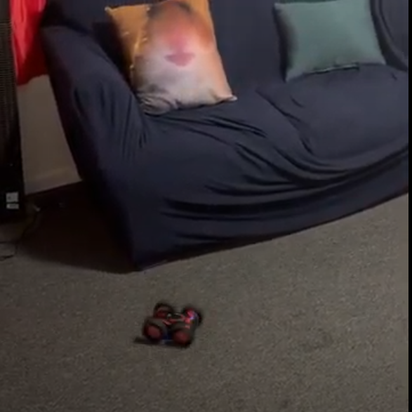
To finish off this lab, I experimented with driving the robot car with the remote control. I noticed that the robot moves very fast and is very susceptible to flipping over if it accelerates too quickly. The robot is also able to turn very quickly, allowing the user to perform quick spins and drifting. Below is a video of me performing a few basic stunts, specificially a flip and a quick spin:
Acknowledgement
I consulted RealPython.com to assist with creating my FFT plots. I referenced Daria Kot's webpage to assist with debugging my complementary filter. I consulted Adafruit.com to learn about implementing two-point calibration.