Mapping

This lab focuses on mapping a robot's environment using orientation and position data. By placing the robot at different locations in a room, one can rotate it through a full 360 degree turn and measure distance data from multiple TOF sensors. With a bit of post-processing, you can use this data to map obstacles and walls that are in the robot's environment.

Orientation Control

The first step towards mapping the robot's environment was to implement a reliable orientation control. This involved reusing my PID orientation control code from lab 6 with a few changes. I wrote a bluetooth command that instructed the robot to execute PID orientation control multiple times. The robot would rotate roughly 20 degrees, stop and record TOF data, and then rotate again and repeat this cycle. Shown below is the code I wrote to implement this functionality:

case LAB9_ROTATE:{
    float rotation_increment = 20;
    int num_rotations = 18;
    float angle_error = 2;
    INDEX = 0;
    init_PID_yaw();
    measure_DMP_data();
    PIDYAW_SETPOINT = DMP_YAW; // set initial setpoint to current orientation

    for(int i = 0; i < num_rotations; i++){
        init_PID_yaw();
        myICM.resetFIFO();
        do{
            runPIDOrientationControl();
        }while(abs(PIDYAW_ERROR) > angle_error);

        stop_motors();
        delay(1500);
        RECORD_MAP();

        PIDYAW_SETPOINT += rotation_increment;
        if(PIDYAW_SETPOINT > 180){
            PIDYAW_SETPOINT -= 360;
        }
        if(PIDYAW_SETPOINT < -180){
            PIDYAW_SETPOINT += 360;
        }
    }
    stop_motors();
    for(int i = 0; i < INDEX; i++){ // If array does not fill in alloted time, only send recorded values and not empty indicies
        tx_estring_value.clear();
        tx_estring_value.append(tof1_stamps[i]);
        tx_estring_value.append("|");
        tx_estring_value.append(tof2_stamps[i]);
        tx_estring_value.append("|");
        tx_estring_value.append(yaw_array[i]);
        tx_characteristic_string.writeValue(tx_estring_value.c_str());
    }
    break;
}

As mentioned previously, the robot would rotate 20 degrees using PID control. The robot would stop rotating when it reached a yaw measurement within 2 degrees of its desired setpoint. Once the robot had rotated to its desired position, it would record 5 distance measurements from each TOF sensor. For this lab, I placed both TOF sensors on the front of the robot. This resulted in a total of 18 rotations per location and 90 distance data points.

While I had implemented wrapping control in lab 6 to prevent large error spikes when the DMP crosses the +- 180 degree threshold, I added control statements to prevent the setpoint from being set to an angle outside of the DMP's measurement range. Additionally, I reset specific PID variables, such as the derivative and integral terms, each rotation in order for the robot to move correctly. I also reset the DMP's FIFO buffer each rotation. When I did not do this, my robot would behave in unexpected ways and would spiral out of control. By resetting the buffer, I ensured that the data I was reading from the DMP was accurate. Lastly, I sent the recorded data to my PC using bluetooth communications. Shown below is my function for recording distance and orientation data:

void RECORD_MAP(){
  measure_DMP_data();
  distanceSensor1.startRanging();
  distanceSensor2.startRanging();
  for(int i = 0; i < 5; i++){
    while(!distanceSensor1.checkForDataReady()){

    }
    while(!distanceSensor2.checkForDataReady()){
      
    }
    tof1_stamps[INDEX] = distanceSensor1.getDistance();
    tof2_stamps[INDEX] = distanceSensor2.getDistance();
    yaw_array[INDEX] = DMP_YAW;
    distanceSensor1.clearInterrupt();
    distanceSensor2.clearInterrupt();
    INDEX += 1;
  }
  distanceSensor1.stopRanging();
  distanceSensor2.stopRanging();
}

For this controller, I used the following constants. KP: 0.2, KI: 0.1, KD: 0.1. I also used a minimum speed of 34%, as the robot would not turn when driven at a speed lower than this threshold. Shown below is a video of my robot performing an on-axis turn:

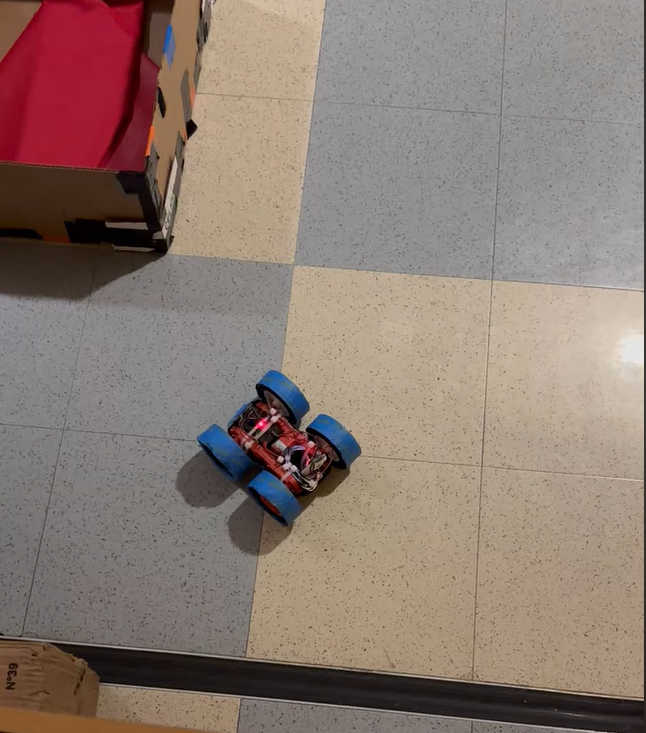
While my robot stayed very close to an on-axis turn, it experienced a bit of drift. Notably, the left wheels of my robot require slightly more power to turn than the right wheels, causing the robot to move in a non-perfect on-axis turn. Instead, it drifts in a circular motion. Through each data recording test, I measured the average drift to be about 1.5 inches. This means that the center of the robot moves about 1.5 inches from its starting location as the robot completes a full rotation. This equates to 38.1 millimeters. With this, I would expect a maximum error of 1.5 inches on my measured map, and an average error of 0.75 inches in a 4x4 meter room.

Map and Obstacle Setup

As I had a lot of difficulty with getting my orientation control to perform correctly (the FIFO buffer on the DMP caused a lot of trouble for me), I wasn't able to record data in the map setup in the lab. Fortunately, I worked with a few other students to create our own map setup on the second floor of Phillips/Duffield Hall.

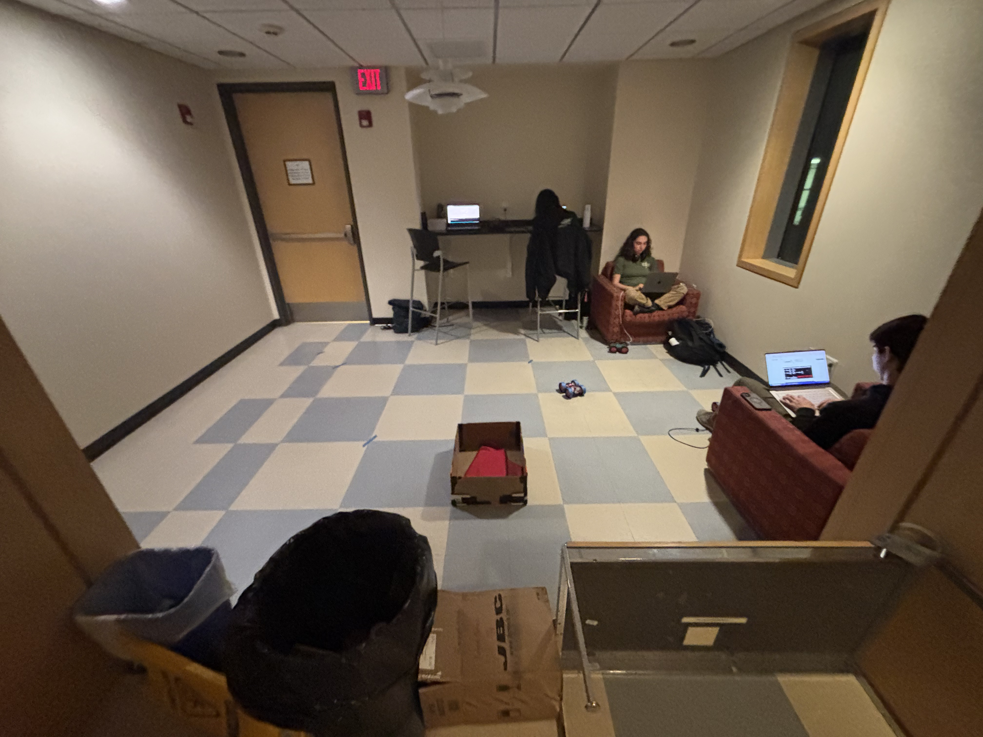
Shown below is an idealized map of our setup, along with a real life photo of our location.

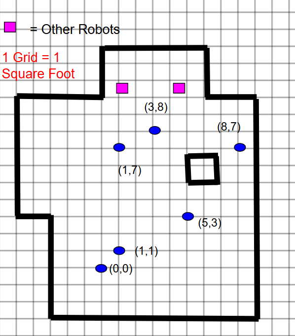
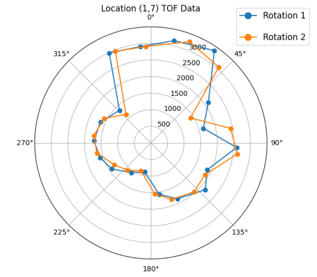
I measured data for each blue point on the map except for the origin (0,0) for a total of 5 locations. At each location, I completed two full rotations. I recorded data from two front-facing TOF sensors. I also started my robot facing in the same direction during each test. At each orientation, I collected 5 data points from each sensor.

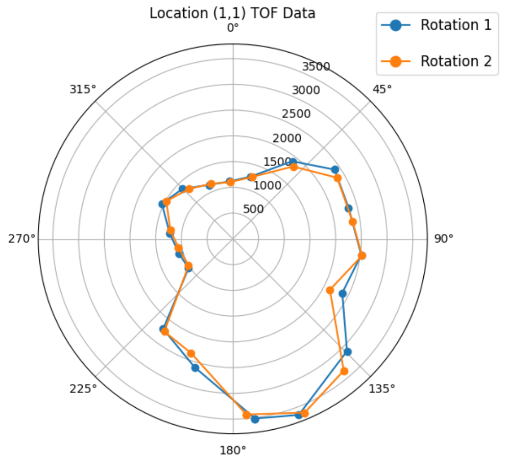
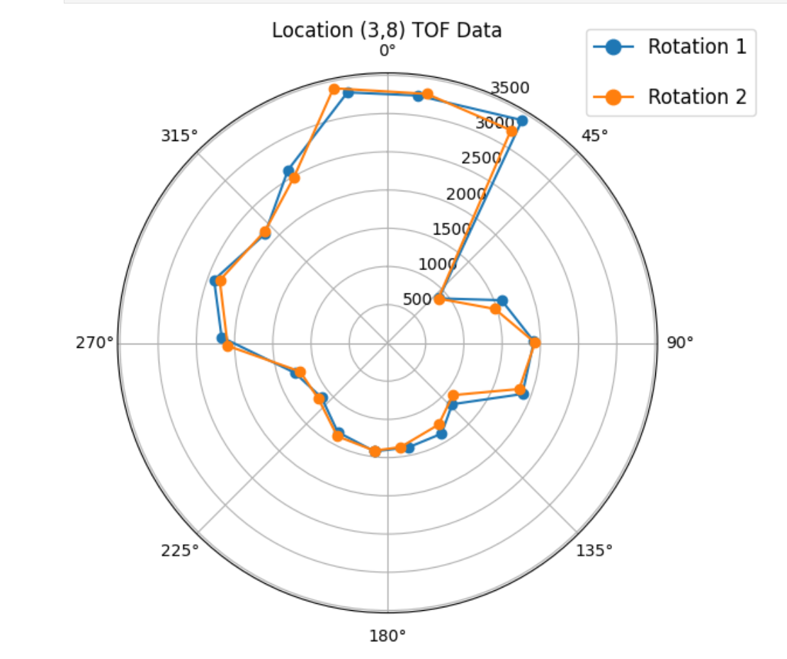
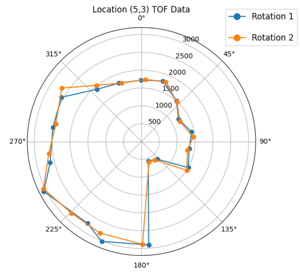
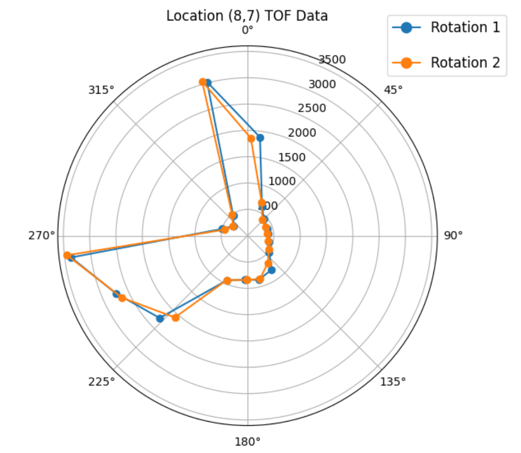
To process this data, I began by averaging the data from each sensor at each orientation, so each full rotation would have 18 averaged data points. Since each location had 2 rotations, this results in 36 averaged data points per location. Since the TOF sensors are on the front of the robot, this is about 76.2 mm away from the center of the robot. I added this distance accordingly to each measurement to account from the distance from the center of the robot. Shown below are polar plots for the data recorded at each location:

Putting it all Together

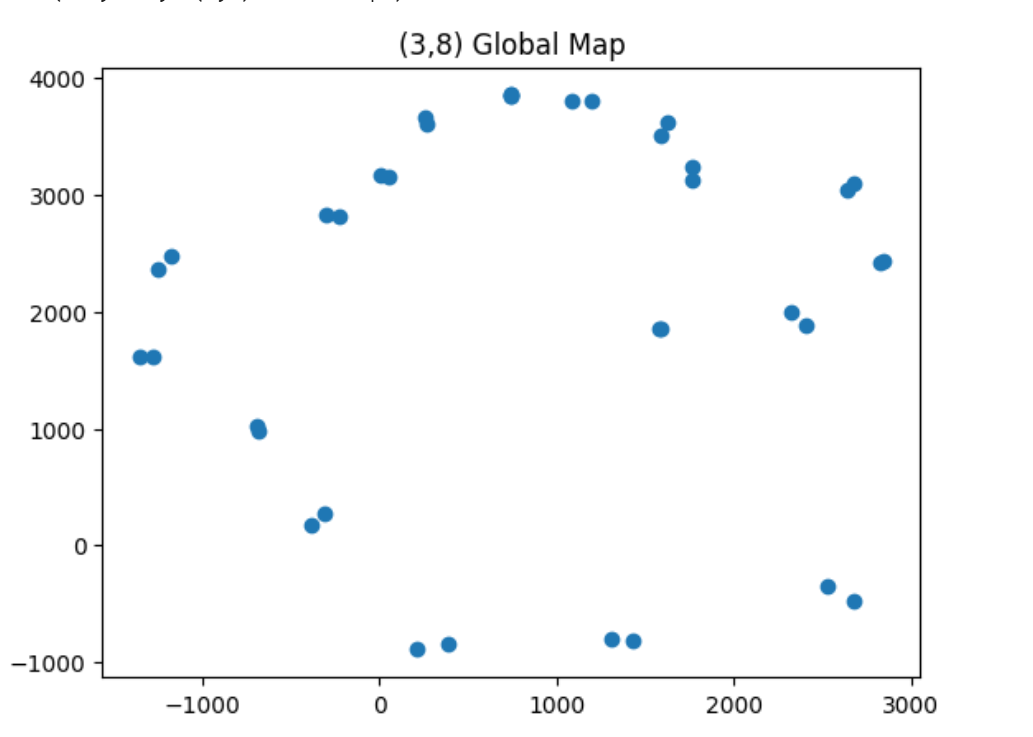
Now that I had distance data for each location, I used transformation matricies to convert the data from each location into a global map. To begin, I converted all of my angle measurements into radians. Since the DMP records angles in degrees, I needed to convert my raw values. To do this, I used the NumPy deg2rad() function.

Next, I applied the following matrix equation to each measurement:

Where theta is the orientation of the robot measured in degrees, and P1 is a column vector consisting of the TOF measurement and an entry of 0. This transformation converted each (theta, distance) measurement into an (x,y) measurement with the robot's center as the origin. Since the robot recorded data at several locations that were not the origin of my map, I needed to add this distance to each transformation.

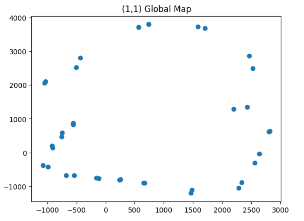
My map records points in measurements of 1 foot (304.8 mm). For example, the point (1,7) would be a distance (304.8, 2133.6) mm away from the origin reference.

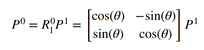
With these transformations complete, we can plot the global map for measured from each of the five locations, as shown below:

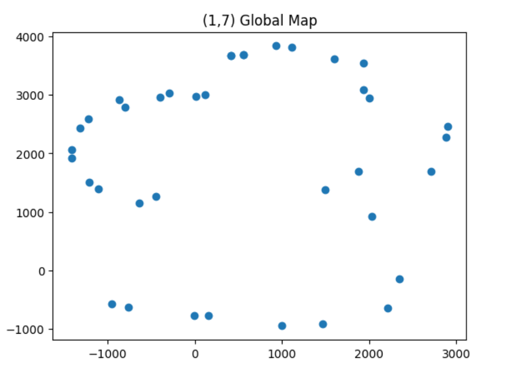
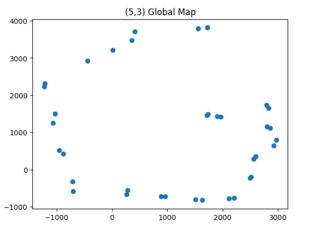
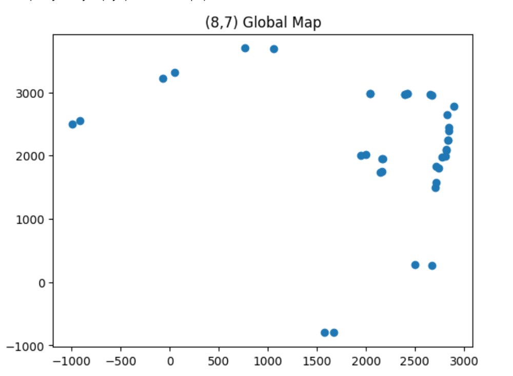
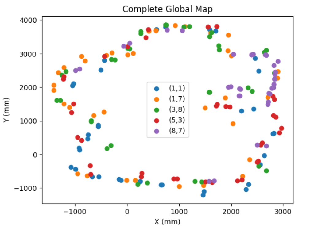
Finally, we can plot each global map together, with a different color representing data from each distinct location. The complete map can be seen below:

If we add lines to the edges of this map, we can see a shape that resembles the original ideal version of the location:

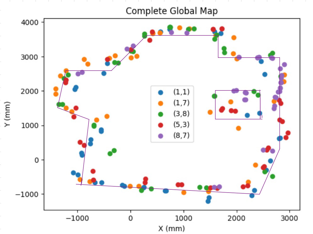
Obviously, the measured map is not perfect. This is due to a few reasons. First, the sensor measurements are not perfect, and there will always be some error in each measurement. Second, there were many objects that moved around slightly or were present in addition to the walls of the created map room. In the previous image of the environment shown above, you can see chairs, backpacks, and people are present. Likely, the TOF sensors recorded these obstacles, resulting in the measured map shown above. However, the measured map is fairly similar to the ideal setup, so I would say that this exercise was a success (although I am biased in that assessment). Overall, this lab was very interesting to work on. After I got through the hurdle of being able to read accurate data from my robot's DMP, the rest of the lab was very satisfying to work on. I look forward to repeating this exercise with the map setup in lab, which will be used in future labs for localization and path planning exercises.

Acknowledgements

I worked with Rachel Arena, Tyler Wisniewski, and Kelvin Resch to create an obstacle setup on the second floor of Phillips Hall. I referenced Daria Kot's and Nila Narayan's webpages, as well as the lecture notes, to develop a better understanding of matrix transformations. I extensively referenced the Matplotlib documentation while writing code for each of the graphs present in this report.